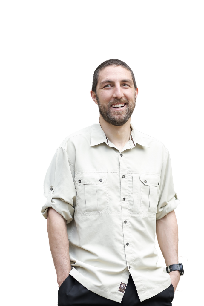
adult-3064693_1920

Happiness in the World – Data Analysis

Happiness in the World – Data Analysis

Introduction:

I wrote Happiness in the World – Data Analysis because I wanted to put data behind what everyone is trying to answer. How to be happy? Happiness is one of the most sought-after things in the world. People get educated, follow their passion, network, make money, help others, all in the pursuit of being happy. Happiness is defined differently depending on who you ask. Maybe one of the most important factors to being happy is your environment. Your environment is something you interact with daily. You craft your environment whether you are stuck in one country or fortunate to experience many countries. In this case, it would not be a stretch to ask if trust in your government determines whether you are happy or not? Maybe a more significant question is if a country is associated with a big cluster. Do each of the clusters show significant variables that help determine a better or worse outcome? A study was conducted to investigate these questions and to determine what effect an environment could have on a person’s happiness.

Happiest Countries in the World:

The data for this test was gathered from sources easily accessible by basic google searches or by going to kaggle.com. The variables within this data are Country, Region, Happiness Rank, Happiness Score, Economy (GDP per Capita), Family, Health (Life Expectancy), Freedom, Trust (Government Corruption), Generosity, Dystopia Residual. The data set contains over 300 observations per variable, all data was compiled by the Sustainable Development Solutions Network. 2017 and 2016 data was analyzed. 2017 because it is most recent and 2016 because it gives a one-year historical view to solidify the results of the analysis further. 2015 data was available but left out since the variables were slightly different and could not be compared accurately to 2016 and 2017.

The initial approach was to create clusters of the data labeled by country. By doing this it is easier for anyone to look at the data point and determine its meaning. It also helps us sort out commonality to draw conclusions. Further analysis was done on the clusters with a Multiple Linear Regression (MLR) Model. Where the clusters were being proved by the variables. By doing this it shows us what variables make the cluster more or less likely to be happy. The third and final analysis was done by proving government trust against all variables, in an MLR model. Trying to prove trust will help us solidify what determines government trust as it is a significant factor in a countries overall happiness.

The analysis of all three methods was done using JMP which is produced by SAS.

Cluster Analysis

The cluster analysis was done by placing the country name in the label position. After the label was set all other variables were sent through the model. It was found that 7 clusters were optimal see Exhibit A:

[image_hover image=’https://enricocecala.com/wp-content/uploads/2018/01/Exa.png’ hover_image=” link=” target=’undefined’ animation=’undefined’ transition_delay=”]

Exhibit A shows us that separation between the clusters is significant enough to warrant analysis. If in fact Exhibit A showed the majority of lines running closely together more clusters would be necessary. Separation is a good sign and shows there is a difference. The difference is important with a cluster it helps us confidently draw a conclusion about the characteristics. Further visuals of the cluster are shown in Exhibit B:

[image_hover image=’https://enricocecala.com/wp-content/uploads/2018/01/Exb.png’ hover_image=” link=” target=’undefined’ animation=’undefined’ transition_delay=”]

Exhibit B shows the clusters against each other. More specifically it shows us where clusters are very different from one another. Why is this important? When looking at Exhibit B we look for clusters pulling away. Pulling away suggests that a cluster is more different than the other clusters. Furthermore, when a cluster is pulling away we can be confident in the cluster being different enough to form a conclusion. For example, where Happiness Score and Generosity cross you can see the purple cluster pulling away. Which means this is a point where the purple cluster is different enough to split from other clusters. What does this mean? Data within the purple cluster as a unit are closely related but different enough from other clusters. If you explore Exhibit B further you will notice more of these separations. The row of Trust is a very dynamic row, it has a lot of dissimilar activity going on. Furthermore, this could mean happiness by country may be determined by the people’s trust. Which is why we will be testing trust specifically.

[image_hover image=’https://enricocecala.com/wp-content/uploads/2018/01/Exc.png’ hover_image=” link=” target=’undefined’ animation=’undefined’ transition_delay=”]

These means in Exhibit C are in cluster order so the top is 1 and then descending to 7. By looking at the data we have good separations between clusters. Happiness Rank from cluster 1 to 2 has a gap of 39. More importantly between these two Cluster 1 is around 1 point higher in happiness then Cluster 2. Furthermore, Cluster 7 is 3 points lower. But Why?  Further analysis shows that Mean(Family) is .664 and Mean(Life Expectancy) is .214 in Cluster 7. Compare these numbers to Cluster 1 Mean(Family) 1.26 and Mean(Life Expectancy) .822. These numbers are double and almost quadruple, cluster 7. You can see how and why these clusters were determined. There are drastic differences between relationships throughout the clusters in many cases.

Putting a Name on the Clusters:

Cluster 1: Freedom Fighters Mean(Freedom) .56, this is much higher than most.

Cluster 2: Non-Generous Mean(Generosity) .17, this is the lowest in the group.

Cluster 3: Family Planners Mean(Family) 1.22, Only second to Cluster 1 by a small margin.

Cluster 4: Government Haters Mean(Government Trust) .07, Lowest in the group.

Cluster 5: Making Family Important Mean(Family) .95, Very close to 3rd overall.

Cluster 6: Terrible Place Mean(Dystopia) 1.48, Lowest score meaning very unpleasant

Cluster 7: Short-Lived Mean(Life Expectancy) .21, Lowest score overall.

The clusters have helped us define the big picture between 7 segregations. But what if we as a country wanted to determine the significance of the variables that determine a cluster. Why is this important? It is important because as a country you can see what factors are important. By doing this you can construct a plan to facilitate a happier environment.

Cluster Multiple Linear Regression (MLR)

[image_hover image=’https://enricocecala.com/wp-content/uploads/2018/01/Exd.png’ hover_image=” link=” target=’undefined’ animation=’undefined’ transition_delay=”]

To predict the likelihood, your country will be placed in a happier cluster. We have to try and predict what variables matter in this determination. The clusters were placed on the Y axis (dependent variable, the value we are trying to forecast) and all others were placed on the X axis (Independent and helps describe the dependent). Each variable was placed in the model. Furthermore, any variable higher than the alpha = .05 (represents a 95% confidence interval (how confident you are in the results)) was removed one at a time from highest to lowest (Stepwise method) until the entire MLR was below the alpha. The result of this process is shown in Exhibit D.


Breaking down Exhibit D from the top and ending at parameter estimates. Within Summary of Fit, there is one value to be concerned with, RSquare Adj. = .88. .88 tells us that the model explains 88% of the question. 88% is a good sign and we can be confident to move further into the analysis. The Analysis of Variance shows us how significant the entire model is and we focus on Prob > F.  Furthermore, with a Prob > F value of <.0001 which is much less than our alpha = .05 we can say the model is significant. We then move down to Parameter Estimates, the intercept is our Y = Clusters, and Prob>|t| is how we determine the significance of a variable by variable scale. You can see all variables are significant except Trust. However, we do not throw this out because there is an interaction term between trust and generosity. Interaction means that the variables interact with one another and helps define how the prediction should look. Since the interaction is significant we cannot get rid of trust. One last thing to check before displaying and using the prediction equation is to check the residual plot. Exhibit E shows the Residual Plot

[image_hover image=’https://enricocecala.com/wp-content/uploads/2018/01/Exe.png’ hover_image=” link=” target=’undefined’ animation=’undefined’ transition_delay=”]

Exhibit E (Residual Plot) identifies if there is a non-random pattern and or a noticeable curve throughout the data. If there are any of these things we can do a quadratic model to try and stabilize the model. The Residual Plot above looks evenly distributed and random. Furthermore, we can be confident about using the prediction equation displayed below.

The resulting prediction equation is:

Y = -3.613555 + .0497576(H Rank) + 1.0090224(H Score) -.714601(Economy) – 2.750078(Health) – .762687(Trust) + 2.0595197(Generosity) + (-.130418475(Trust))*           (-.2447455708(Generosity)*-10.93921)

Explaining Government Trust

The scatter plot for the clusters showed that Trust was something very important in the determination. Trust was a variable that helped decide a countries cluster. It is not hard to believe that trust in how your country is administered has such a huge effect on happiness. The variable has a huge influence on how you live, sleep, eat, and breath. That is why it is so important to try and figure out what creates a harmonious government in the pursuit of happiness. The technique to determine Trust was using the MLR method. All the same, rules apply, that were applied above. 95% confidence, anything above Alpha = .05 was thrown out.

[image_hover image=’https://enricocecala.com/wp-content/uploads/2018/01/Exf.png’ hover_image=” link=” target=’undefined’ animation=’undefined’ transition_delay=”]

Exhibit F’s RSquare Adj is .99 meaning 99% of the story is determined in this model. This is extremely high and should add a layer of comfort going forward. The Analysis of Variance (ANOVA) is Prob > F = <.0001 which is much less than our alpha. To continue into the Parameter Estimates the Intercept = Trust (our Y). All variables are very significant well below our Alpha = .05. We then look to the Residual Plot to ensure randomness and normal distribution.

[image_hover image=’https://enricocecala.com/wp-content/uploads/2018/01/Exg.png’ hover_image=” link=” target=’undefined’ animation=’undefined’ transition_delay=”]

As you can see in the residual plot has randomness and a normal distribution of points. We can now display the equation to predict trust:

Y = -.000134 + 1.0002613(H Score) – 1.000295(Economy) – 1.000238(Family) – 1.00015(Health) – 1.00035(Freedom) – 1.000448(Generosity) – 1.00021(Dystopia)

Unhappiest Country in the World

This model shows a very clear picture of what is important in the trust of government. In the Cluster analysis, one of the major factors in the determination of happiness was trust. If the government is corrupted or untrustworthy how could you live peacefully in your environment? Bulgaria is in cluster 4 was called Government Haters has one of the lowest trust scores of .006 and a Dystopia lower than the lowest cluster score. It is obviously not a very happy place. All three of these tests are important to help start the conversation about building a stronger happier world.

Recommendations:

The data was straightforward and clear enough administer analysis. But there could be improvements. First and foremost, who collects the data should hold to the standards initially set forth. 2015 data columns were different than 2016 and 2017. Since they were grossly different 2015 was not incorporated. Furthermore, by not being able to run 2015 data we miss out on further insight into the mystery of happiness. The data can become more robust as well. Determining the ratio of wealthy, mid, and lower-class citizens in a country would be interesting to put into a model. Furthermore, the ratio of educated people to non-educated, and crime per capita. These factors would need further definition to determine what does educated mean and what determines wealthy. However, it is worth factoring into the model to fully understand the people who live in the countries being studied. We might see a country that is uneducated is unhappy because they are easily oppressed. The data tells a very high-level view of the overall happiness field and neglects the finer personal detail needed for such a determination.

In Conclusion:

Happiness is one of the most sought-after goals on the planet. When you are happy time flies, you are carefree, less worried, boost immunity, and the list goes on. The variables to determine happiness will need to be consistently evolved and tracked. Data presented in this report is only the beginning of a more detailed analysis that needs to take place. It is clear however that happiness can be spearheaded by how trusting the citizens are of their government. Furthermore, this could lead into a much bigger discussion, about educational support, diversity support, minority support, and the ability to be a free thinker.

More Visuals for those visual learners out there:

[image_hover image=’https://enricocecala.com/wp-content/uploads/2018/01/Encl1.png’ hover_image=” link=” target=’undefined’ animation=’undefined’ transition_delay=”]

[image_hover image=’https://enricocecala.com/wp-content/uploads/2018/01/Encl2.png’ hover_image=” link=” target=’undefined’ animation=’undefined’ transition_delay=”]

[image_hover image=’https://enricocecala.com/wp-content/uploads/2018/01/Encl3.png’ hover_image=” link=” target=’undefined’ animation=’undefined’ transition_delay=”]

***A higher score in Dystopia means it is more pleasant. ***

[image_hover image=’https://enricocecala.com/wp-content/uploads/2018/01/Encl4.png’ hover_image=” link=” target=’undefined’ animation=’undefined’ transition_delay=”]

[image_hover image=’https://enricocecala.com/wp-content/uploads/2018/01/Encl5.png’ hover_image=” link=” target=’undefined’ animation=’undefined’ transition_delay=”]

Share this post

Leave a comment

Your email address will not be published. Required fields are marked *